Understanding radioactive decay is fundamental to fields ranging from archaeology to medicine, yet the mathematics behind it often induces unnecessary anxiety. For researchers attempting to determine the age of an artifact or the safety window for a medical isotope, knowing how to solve half-life problems is a non-negotiable skill. The process does not require advanced calculus, but it does demand a rigorous approach to algebra and a clear understanding of exponential functions. By breaking down the problem into manageable variables, you can accurately model the decay of any substance.
When You Need to Establish the Formula Framework
The foundation of every successful calculation lies in selecting the correct model. The standard half-life equation, $N(t) = N_0 \cdot (1/2)^t/t_1/2$, relates the remaining quantity of a substance to its initial amount and the elapsed time. To utilize this effectively, you must first identify your known variables: the initial mass ($N_0$), the final mass ($N(t)$), the half-life of the isotope ($t_1/2$), and the total time elapsed ($t$). A common failure point occurs when researchers mix up the remaining mass with the amount that has decayed; always ensure you input the quantity that is still present at time $t$ for $N(t)$ to avoid logical errors.
When Calculating Remaining Mass After Decay
In many practical laboratory scenarios, the goal is to predict how much of a sample remains after a specific duration. This scenario requires you to solve for $N(t)$. The benefit of this calculation is evident in quality control processes, ensuring that materials retain necessary properties over time. To proceed, simply substitute the known time and the isotope’s specific half-life into the exponent. However, exercise caution: the unit of time used for the elapsed period must match the unit of the half-life. If the half-life is given in years and your time span is in days, you must convert the days to years before calculating. A mismatch in units is the most frequent cause of order-of-magnitude errors in these problems.
When Solving for Elapsed Time
Conversely, you may know the starting and ending quantities but need to determine how long the process has taken. This is a typical requirement in geochronology or forensic analysis. Solving for time introduces a layer of complexity because the variable $t$ is located in the exponent. To isolate it, you must employ logarithms. Taking the natural log ($\ln$) of both sides of the equation allows you to bring the exponent down, transforming the equation into a linear form that is easily solvable. While this step is mathematically sound, it is computationally sensitive; rounding off your logarithmic values too early in the process can significantly skew your final time estimate, so maintain precision through the final step.
When Handling Fractional Half-Lives
Not all decay processes occur in neat, whole-number increments. You will frequently encounter scenarios where the elapsed time is not a perfect multiple of the half-life, resulting in fractional exponents. Researchers should view this as an opportunity for higher precision rather than a hurdle. The math remains identical to the whole-number method, as the exponential function handles fractions seamlessly. The key benefit here is the ability to date events with high granularity. Do not attempt to approximate the time by linearizing the curve; always rely on the exponential nature of the formula. Linear approximation dramatically underestimates the decay rate in the early stages and overestimates it later, leading to flawed conclusions about the sample's history.
Understanding radioactive decay is fundamental to fields ranging from archaeology to medicine, yet the mathematics behind it often induces unnecessary anxiety. For researchers attempting to determine the age of an artifact or the safety window for a medical isotope, knowing how to solve half-life problems is a non-negotiable skill. The process does not require advanced calculus, but it does demand a rigorous approach to algebra and a clear understanding of exponential functions. By breaking down the problem into manageable variables, you can accurately model the decay of any substance.
When You Need to Establish the Formula Framework
The foundation of every successful calculation lies in selecting the correct model. The standard half-life equation, $N(t) = N_0 \cdot (1/2)^t/t_1/2$, relates the remaining quantity of a substance to its initial amount and the elapsed time. To utilize this effectively, you must first identify your known variables: the initial mass ($N_0$), the final mass ($N(t)$), the half-life of the isotope ($t_1/2$), and the total time elapsed ($t$). A common failure point occurs when researchers mix up the remaining mass with the amount that has decayed; always ensure you input the quantity that is still present at time $t$ for $N(t)$ to avoid logical errors.
When Calculating Remaining Mass After Decay
In many practical laboratory scenarios, the goal is to predict how much of a sample remains after a specific duration. This scenario requires you to solve for $N(t)$. The benefit of this calculation is evident in quality control processes, ensuring that materials retain necessary properties over time. To proceed, simply substitute the known time and the isotope’s specific half-life into the exponent. However, exercise caution: the unit of time used for the elapsed period must match the unit of the half-life. If the half-life is given in years and your time span is in days, you must convert the days to years before calculating. A mismatch in units is the most frequent cause of order-of-magnitude errors in these problems.
When Solving for Elapsed Time
Conversely, you may know the starting and ending quantities but need to determine how long the process has taken. This is a typical requirement in geochronology or forensic analysis. Solving for time introduces a layer of complexity because the variable $t$ is located in the exponent. To isolate it, you must employ logarithms. Taking the natural log ($\ln$) of both sides of the equation allows you to bring the exponent down, transforming the equation into a linear form that is easily solvable. While this step is mathematically sound, it is computationally sensitive; rounding off your logarithmic values too early in the process can significantly skew your final time estimate, so maintain precision through the final step.
When Handling Fractional Half-Lives
Not all decay processes occur in neat, whole-number increments. You will frequently encounter scenarios where the elapsed time is not a perfect multiple of the half-life, resulting in fractional exponents. Researchers should view this as an opportunity for higher precision rather than a hurdle. The math remains identical to the whole-number method, as the exponential function handles fractions seamlessly. The key benefit here is the ability to date events with high granularity. Do not attempt to approximate the time by linearizing the curve; always rely on the exponential nature of the formula. Linear approximation dramatically underestimates the decay rate in the early stages and overestimates it later, leading to flawed conclusions about the sample's history.
The 7 Best Android Apps To Help You Solve Math Problems
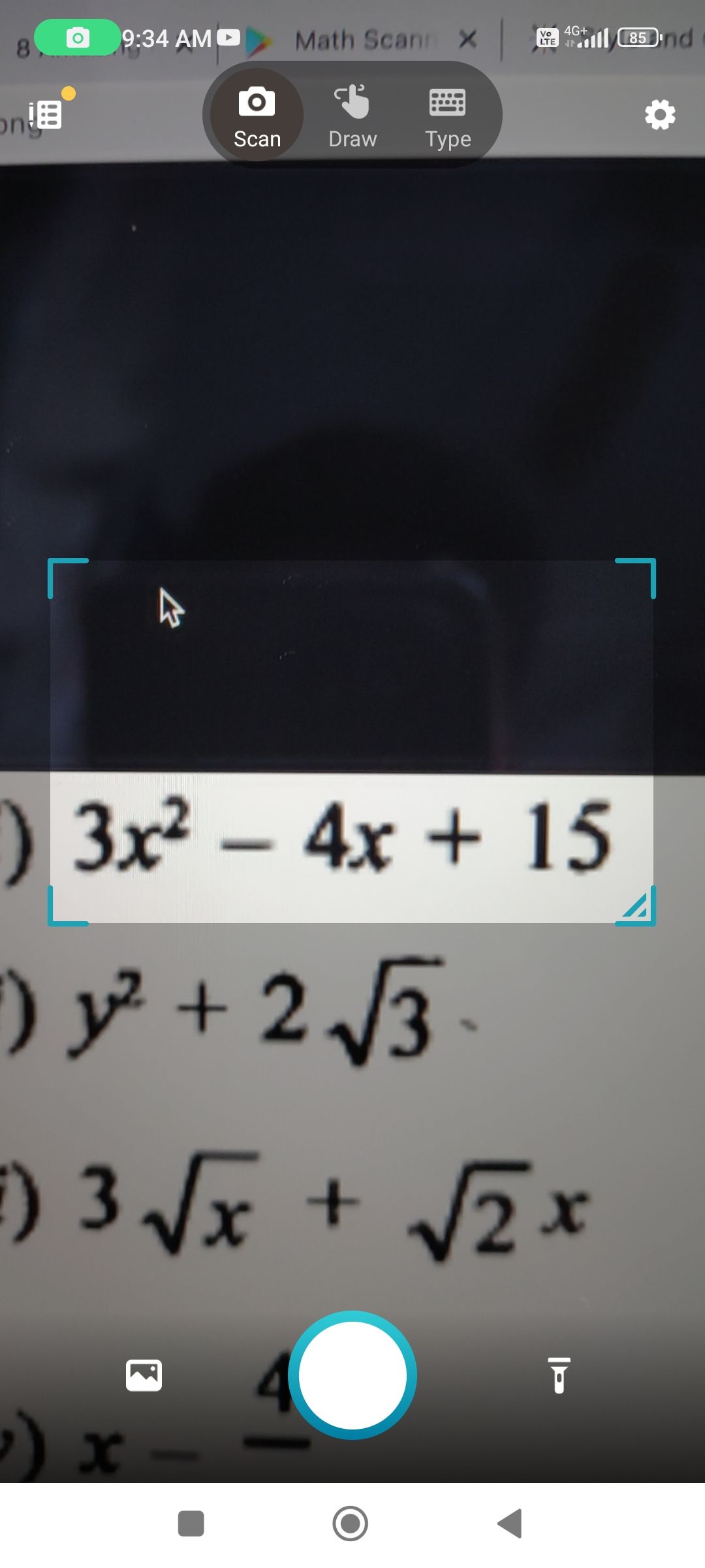
The 7 Best Android Apps to Help You Solve Math Problems
Algebra Problem Solver: Can You Solve This Equation?

Algebra Problem Solver: Can You Solve This Equation?
Math Problem Solver

Math Problem Solver